Natural Language Processing
Explore the fundamental techniques that transform human language into machine-understandable representations. From simple word counting to advanced semantic embeddings, these methods form the backbone of modern NLP applications.
Example Text Corpus
- Machine learning is fascinating
- Deep learning advances machine learning
- Natural language processing uses machine learning
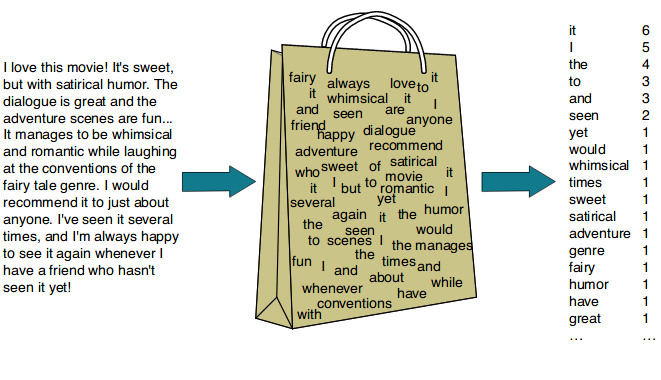
Bag of Words (BoW)
Concept
The Bag of Words model converts text into numerical features by counting word occurrences. It ignores grammar and word order but keeps frequency information. Each unique word in the corpus becomes a feature, creating a vocabulary-based vector representation.
Vocabulary
["advances", "deep", "fascinating", "is", "language", "learning", "machine", "natural", "processing", "uses"]Example
Sentence: "Machine learning is fascinating"
Tokens: ["machine", "learning", "is", "fascinating"]
Vector Representation
Sentence 1: "Machine learning is fascinating"
[0, 0, 1, 1, 0, 1, 1, 0, 0, 0]

Sentence 2: "Deep learning advances machine learning"
[1, 1, 0, 0, 0, 1, 1, 0, 0, 0]

Sentence 3: "Natural language processing uses machine learning"
[0, 0, 0, 0, 1, 1, 1, 1, 1, 1]- Only word counts matter - no context or meaning captured
- "learning" appears in all sentences with a count of 1
- No sense of word order or grammar
- Creates sparse vectors (many zeros)
- Simple and fast but loses semantic information
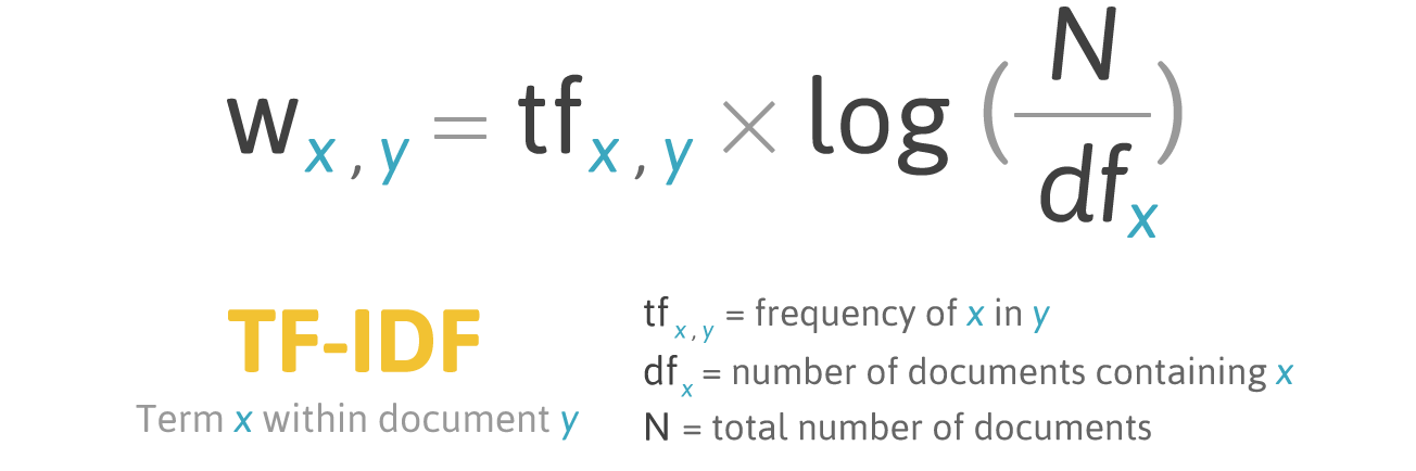
TF-IDF (Term Frequency–Inverse Document Frequency)
Concept
TF-IDF measures how important a word is in a document relative to the entire corpus. Common words that appear in many documents get low scores, while unique words that appear in few documents get high scores. This helps identify distinctive terms for each document.
Formula
$$ \text{TF-IDF}(t, d) = \text{TF}(t, d) \times \log\left(\frac{N}{n_t}\right) $$
Where:
- TF(t, d) = Term Frequency of term t in document d
- N = Total number of documents
- nt = Number of documents containing term t
Example Calculation
Suppose the word "fascinating" appears once in a 4-word document and appears in only 1 out of 3 documents:
TF(fascinating) = 1 / 4 = 0.25
IDF(fascinating) = log(3 / 1) = 1.098
TF-IDF = 0.25 × 1.098 = 0.2745
Vector Representation (Approximate Values)
Sentence 1:
[0, 0, 0.58, 0.46, 0, 0.40, 0.40, 0, 0, 0]

Sentence 2:
[0.58, 0.58, 0, 0, 0, 0.33, 0.33, 0, 0, 0]

Sentence 3:
[0, 0, 0, 0, 0.37, 0.29, 0.29, 0.37, 0.37, 0.37]- "fascinating" (unique word) has high weight → 0.58
- "learning" and "machine" (common words) have lower weight → 0.29–0.40
- Produces weighted sparse vectors
- Highlights document-specific and unique terms
- Better than BoW for information retrieval tasks
Word2Vec (Semantic Embeddings)
Concept
Word2Vec learns dense numeric representations of words (embeddings) by analyzing their contexts in large text corpora. Words that occur in similar surroundings end up with similar vectors in a multi-dimensional space. It uses either the Skip-Gram (predict context from word) or CBOW (Continuous Bag of Words - predict word from context) approach.
How It Works
Word2Vec creates dense vectors (typically 100–300 dimensions) where semantic relationships are encoded geometrically. Similar words have vectors that point in similar directions, and mathematical operations on vectors preserve meaningful relationships.
Example Context Learning
Sentence: "The king and queen rule the kingdom"
Both "king" and "queen" appear in similar contexts (with words like "rule" and "kingdom"), so their vectors become similar in the embedding space.
Individual Word Vectors (First 5 of ~100 dimensions)
Word         Vector Representation
machine      [ 0.12, -0.23,  0.44,  0.01, -0.35, ...]
learning     [ 0.15, -0.20,  0.47,  0.05, -0.30, ...]
deep         [ 0.42, -0.55,  0.33,  0.12, -0.09, ...]
natural      [-0.18,  0.22,  0.66, -0.04,  0.20, ...]
processing   [-0.15,  0.25,  0.63, -0.03,  0.18, ...]
Semantic Relationships
Each vector encodes semantic relationships, enabling powerful operations:
cosine_similarity("machine", "learning")→ high similarity (words used together)cosine_similarity("machine", "banana")→ low similarity (unrelated concepts)- Vector arithmetic:
king - man + woman ≈ queen - Finding analogies:
Paris - France + Italy ≈ Rome
- Dense vectors (every dimension has a non-zero value)
- Meaningful geometry — direction and distance encode semantic relationships
- Learned automatically from large text corpora (requires substantial data)
- Captures context and semantic meaning, not just frequency
- Enables transfer learning and powers many modern NLP applications
- Can handle synonyms and word analogies naturally
Comprehensive Comparison
| Technique | Representation Type | What It Captures | Example Vector | Advantages | Limitations |
|---|---|---|---|---|---|
| Bag of Words | Sparse count vector | Word presence and frequency | [0, 0, 1, 1, 0, ...] |
Simple, fast, interpretable, works well for small datasets | Ignores meaning, context, word order, and semantic relationships |
| TF-IDF | Weighted sparse vector | Word importance relative to corpus | [0.58, 0, 0.33, ...] |
Highlights unique words, reduces common word impact, better for search and classification | Still ignores semantic meaning, context, and word relationships |
| Word2Vec | Dense semantic vector | Contextual meaning and semantic relations | [0.12, -0.23, 0.44, ...] |
Captures deep semantics, enables analogies, context-aware, supports transfer learning | Requires large datasets, computationally expensive to train, less interpretable |
Summary
- Bag of Words counts words and creates simple frequency-based representations — great for basic text analysis
- TF-IDF values words by their importance across documents — ideal for information retrieval and document classification
- Word2Vec understands words through learned semantic relationships and contextual meaning — powers advanced NLP applications like sentiment analysis, machine translation, and question answering
The evolution from BoW to Word2Vec represents the journey from simple statistical methods to deep learning approaches in Natural Language Processing, each serving different use cases and computational requirements.